How To Read The Transient Response In Matlab Low Pass Filter Voltage Gain

Activeness i Part (b): Frequency-Response Identification of a Resistor–Capacitor (RC) Circuit

Key Topics: Modeling Electrical Systems, First-Lodge Systems, Arrangement Identification, Frequency Response, Bode Plots

Equipment needed
Purpose
Theoretical frequency response
Organization identification experiment
Information acquisition
Extensions

Equipment needed

Arduino board (e.one thousand. Uno, Mega 2560, etc.)
Breadboard
Electronic components (resistor and capacitor)
Ohmmeter, Capacitance meter (optional)
Jumper wires

Following up the Activity 1a, nosotros volition employ the same Resistor–Capacitor (RC) Circuit in this experiment. The hardware and software needed for this experiment volition as well be the same as used previously. Specifically, the Arduino board volition be used for generating the input to the excursion and for measuring the output of the ciruit. The input to the excursion will exist generated from one of the board's Digital Outputs, applied beyond the resistor and capacitor in series. The output of the circuit will exist the voltage across the capacitor which will be read via one of the board's Analog Inputs. This data is then fed to Simulink for visualization and for comparison to our theoretical predictions.

Purpose

In the previous activity nosotros examined the fourth dimension response of an RC circuit. The purpose of this activity is rather to understand the frequency response of the same circuit. Specifically, we are going to experimentally construct the magnitude plot portion of the Bode plot for the RC circuit. In this action we will sweep through a range of frequencies, but nosotros will employ square wave inputs rather than sine wave inputs. In this regard, the magnitude response that we generate won't exactly correspond to the standard definition of frequency response. The reason we will employ square wave inputs is to build intuition regarding the meaning of the circuit'due south frequency response based on the understanding of the circuit's step response we gained in Activeness 1a.

Theoretical frequency response

The thought behind frequency response assay is to examine how a organisation responds to sinusoidally varying inputs of unlike frequencies. If we take a linear system, as we do in this example, and so a sinusoidal input of a item frequency will generate in steady-state a sinusoidal output of the same frequency. The output, however, may have a unlike amplitude than the input and the output may be stage shifted as compared to the input. This idea is demonstrated below.

One tin understand the higher up by considering that if our system is represented as the transfer function $G(s)$ , then the output is only the product of the transfer part and the input, $Y(s) = G(s)R(s)$ . Therefore, the output can be separated (via a partial fraction expansion) into a component with the poles of the transfer function (representing the arrangement'south natural response) and a component with the poles of the input betoken. If the organisation is stable, and so the natural response will dice out resulting in a steady-state output that has the same form (poles) every bit the input indicate.

When we consider a organization's frequency response, we are specifically interested in how the amplitude and phase of the steady-land output compare to the sinusoidal input. One manner to represent this amplitude (magnitude) data and this phase data is equally a Bode plot. A Bode plot consists of 2 graphs, i existence the magnitude of the response (the ratio of the output aamplitude to the input aamplitude, $Y/R$ ) versus frequency, and the other existence the phase of the response versus frequency.

Executing the post-obit commands at the MATLAB control line will generate the theoretical Bode plot for our RC circuit (with $R = 10 k\Omega$ , $C = 100 \mu F$ ).

south = tf('s'); R = 10000;                                         C = 100*10^-6;                                     G = 1/(C*R*southward+1);                                   bode(G) championship('RC Excursion Frequency Response (R = ten kOhm, C = 100 uF)')

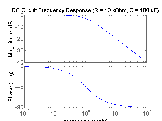
Exam of the above demonstrates that the RC circuit behaves similar a low-pass filter (passes low frequencies and blocks high frequencies). At depression frequencies, the circuit has a magnitude response of zero decibels. Recall that in decibels the magnitude is calculated as $20 \log Y/R$ , therefore, a magnitude of 0 dB corresponds to the instance that the output amplitude is equal to the input amplitude (the ratio $Y/R$ equals ane). While at higher frequencies, the magnitude in dBs becomes more and more negative. This tendency corresponds to the amplitude ratio becoming closer to zero, that is, the output is adulterate to a greater degree as the input frequency is increased. The trend observed in the phase plot is that the output lags behind the input to greater caste every bit the input frequency is increased.

These trends are observed in most physical systems. As the frequency of the input increases, the organisation has a harder fourth dimension "keeping up" with the input. Through the form of the hardware experiment in the side by side section, we will endeavor to build some intuition for this phenomenon. In the instance of the organisation we are examining here, the frequency at which the input begins to be attenuated is determined by the size of the electronic components $R$ and $C$ . Specifically, recall the transfer function for the RC circuit:

(1) $G(s) = \frac{E_o(s)}{E_i(s)} = \frac{1}{RCs+1} = \frac{K}{\tau s+1}$

The break frequency for this excursion is determined by the location of its pole, that is, the intermission frequency equals $1/\tau = 1/RC$ . In the case of this excursion, $RC = 1$ and the suspension frequency is in the neighborhood of 1 rad/sec. Recalling the course of the RC circuit'south step response, we can anticipate how the circuit volition respond to a square wave input of varying frequencies. We will verify our intuition with a hardware-based experiment in the next section. The overall purpose of this activity is to meliorate understand what a system's frequency response means.

Executing the following commands at the MATLAB command line will generate the theoretical step response plot for our RC excursion (with $R = 10 k\Omega$ , $C = 100 \mu F$ ).

s = tf('s'); R = 10000;                                         C = 100*10^-6;                                     G = 1/(C*R*south+one);                                   step (Chiliad) championship('RC Excursion Step Response (R = x kOhm, C = 100 uF)')

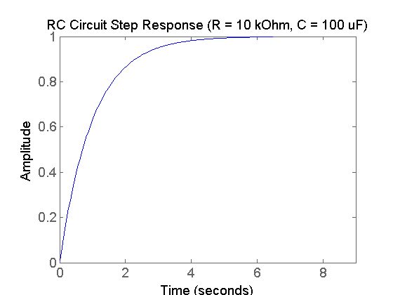
Examination of the above shows a standard commencement-order stride response. For a square wave input, one tin imagine that the output will rise as shown above when the input is "ON" and volition decay exponentially when the input is "OFF." Cycling between the "ON" and "OFF" states will and then generate a response like the one shown below.

In the above figure, the menstruation of the square wave input is sufficiently large that the organization output has time to approximately accomplish steady-state before the input indicate switches its value. Recall that for a first-gild organization, it takes approximately iv fourth dimension constants ( $4\tau$ ) for the output to accomplish $98 \%$ of its total modify. Therefore, when the input frequency is sufficiently irksome (catamenia sufficiently big compared to $\tau$ ) the output response will announced every bit in the in a higher place effigy where the amplitude of the output is approximately equal to the amplitude of the input. This is what was observed in the Bode plot generated earlier. At low frequencies, the magnitude approximately equaled $20\log 1 = 0$ dB, which corresponds to an amplitude ratio of ane (no attenuation).

Further recollect that it takes approximately ane time constant ( $\tau$ ) for a standard first-order footstep response to accomplish $63 \%$ of its total change. Therefore, when the square wave has a menstruation of $2\tau$ (frequency equal $2\pi/2\tau \approx 3.14$ rad/sec for this system) the output response will non have time to reach steady-land before the input switches value again. Equally such, the amplitude of the output will be smaller than the amplitude of the input. This is observed in the previously generated Bode plot in that the magnitude higher up the break frequency (ane rad/sec) is less than 1 (less than 0 dB). As the frequency of the input increases, there is even less time for the output to react. This is indicated in the Bode plot by the fact the system's magnitude (the output amplitude) gets smaller and smaller as the frequency of the input is increased.

Nosotros volition investigate this phenomenon in the following experiment.

System identification experiment

In this experiment we volition record the output voltage of the RC circuit for a square wave voltage input. Specifically, the voltage input will alternating betwixt 0 Volts and 5 Volts, where the time "OFF" will equal the time "ON." The frequency of the foursquare wave input will be varied and the resulting amplitude of the circuit'due south output response will be recorded to approximate the system's magnitude response. In a sense, we are generating the organisation's frequency response model empirically. This is sometimes referred to as a blackbox model or a data-driven model. The hardware and software setup we volition use is very similar to that employed in Part (a) of this activity.

Hardware setup

Our simple RC circuit can be implemented on a breadboard and continued to the Arduino board as shown. Retrieve that if you employ an electrolytic capacitor, its orientation matters. The Arduino board is employed to receive the input voltage command from Simulink and to apply the voltage to the circuit (via a Digital Output). The board as well acquires the output voltage data from the circuit (via an Analog Input) and communicates the data to Simulink.

In this experiment, the values of the resistor and capacitor are called ( $R = 10\ k\Omega$ , $C = 100\ \mu F$ ) such that the excursion's time response is irksome plenty that the Arduino/Simulink setup tin can sample the circuit at a fast enough charge per unit to give a clear picture show of the circuit's output. Since we are generating the circuit'south frequency response, we wish to be able to accurately capture the circuit's response at frequencies at least ane or two decades above the circuit's break frequency (one rad/sec).

Software setup

In this experiment, nosotros will utilise Simulink to read the information from the board and to plot the data in real time. In particular, we will employ the IO packet from the MathWorks. For details on how to use the IO bundle, refer to the following link. The Simulink model nosotros will use in this experiment is substantially the same equally the ane nosotros used in Office (a) of this activity. The model can be downloaded here, where you may need to change the port to which the Arduino board is continued (the port is COM5 in this example).

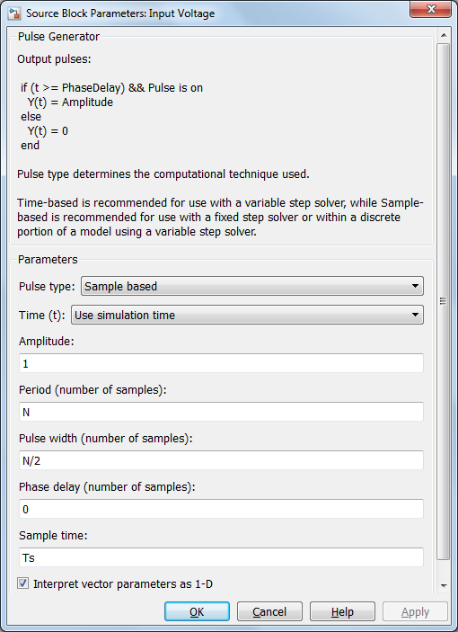
As shown below, the input voltage command is generated by a Pulse Generator block (for generating a square wave input). The Pulse Generator block generates values of 0 or 1 which are then fed to an Arduino Digital Write block. Since nosotros are using channel 8 for the digital output, we double-click on the Arduino Digital Write block to ready the Pin to 8 from the drop-downwardly menu. An input of 0 to the Digital Write cake causes an output of 0 Volts to be generated at the corresponding pin, while an input of i to the Digital Write block generates an output of v Volts. This scaling is captured past the Gain block that is included prior to the Scope block.

The Arduino Analog Read block reads the output voltage information via the Analog Input A0 on the lath. Double-clicking on the block allows u.s.a. to prepare the Pin to 0 from the drop-down carte. We likewise will set the Sample Time based on the frequency of the input being employed. For example, for an input frequency of x rad/sec (1 decade above the circuit's suspension frequency), we could employ a sample fourth dimension of "0.02". This sample time corresponds to a sampling frequency of 50 Hz, which is more than 30 times faster than the frequency of the input signal (10 rad/sec $\approx$ 1.59 Hz). This means the that excursion'southward response for this input would be sampled more thirty times per wheel. This is enough to capture the character of the organisation's output at this frequency. The downloadable model included to a higher place defines all sample times every bit Ts (or left as "-1"). Therefore, before you run this model yous must ascertain the variable Ts in the MATLAB workspace, for example, by typing Ts = 0.02; at the command line. The Gain block is included to catechumen the information into units of Volts (past multiplying the data by 5/1023).

The given Simulink model then plots the commanded input voltage and recorded output voltage on a scope and as well writes the output data to the MATLAB workspace for further analysis. The Arduino Digital Write block, the Arduino Analog Read block, the Arduino IO Setup cake, and the Real-Time Pacer cake are all part of the IO packet. The remaining blocks are part of the standard Simulink library, specifically, they tin be found nether the Math, Sources, and Sinks libraries.

Information acquisition

To experimentally construct a Bode magnitude plot, we volition sweep through a series of square wave inputs of varying frequency and record the amplitude of the output response. In lodge to get a complete moving picture of the RC circuit's frequency response, we need to capture frequencies ranging from at least ane decade beneath the break frequency to at least 1 decade above the pause frequency. Specifically, we volition wait at frequencies ranging from approximately 0.05 rad/sec (20 times smaller than ane rad/sec) all the way upward to about 30 rad/sec (thirty times larger than 1 rad/sec). Below provides a table describing the input signal periods and frequencies, every bit well as the sampling time and duration employed to guarantee the circuit's response is sampled frequently enough and the response is given sufficient fourth dimension to attain steady state.

(2) $\begin{tabular}{l c c c c} &\textbf{T(sec)}&\textbf{freq(rad/sec)}&\textbf{Ts(sec)}&\textbf{Duration(sec)}\\\hline \textbf{(1)}&125&0.050&0.1&300\\ \textbf{(2)}&60&0.105&0.1&100\\ \textbf{(3)}&40&0.157&0.1&100\\ \textbf{(4)}&20&0.314&0.1&40\\ \textbf{(5)}&15&0.419&0.1&40\\ \textbf{(6)}&12&0.524&0.1&40\\ \textbf{(7)}&10&0.628&0.1&40\\ \textbf{(8)}&9&0.698&0.05&40\\ \textbf{(9)}&8&0.785&0.05&40\\ \textbf{(10)}&7&0.898&0.05&40\\ \textbf{(11)}&6&1.047&0.05&40\\ \textbf{(12)}&5&1.257&0.05&40\\ \textbf{(13)}&4&1.571&0.05&40\\ \textbf{(14)}&3&2.094&0.05&40\\ \textbf{(15)}&2&3.142&0.05&40\\ \textbf{(16)}&1&6.283&0.05&40\\ \textbf{(17)}&0.6&10.47&0.02&40\\ \textbf{(18)}&0.4&15.71&0.02&40\\ \textbf{(19)}&0.2&31.42&0.02&40\\ \end{tabular}$

For demonstration purposes, we will look at the excursion's response to a square wave input of menses $T = 4$ seconds. This corresponds to a frequency of approximately i.571 rad/sec, which is slightly faster than the circuit's ane rad/sec interruption frequency. To get started, enter the following commands in the control window:

T=4;       Ts=0.05;   Due north=T/Ts;

At present open (or create) the Simulink model provided earlier in this section. Double-click on the Input Voltage block and the Arduino Analog Read block, respectively, and fix the parameters $N$ and $Ts$ every bit shown beneath.

Earlier running the Simulink model, make sure that its run length is set to xl seconds as shown below, respective to the table that we previously introduced.

Inbound the following code at the MATLAB command line will generate a plot like the one shown below which includes the square moving ridge input and the circuit'southward output response.

          figure; plot(0:Ts:40,eo_act,0:Ts:40,ei,'r');          xlabel('fourth dimension (sec)')          ylabel('signals (Volts)')          championship('RC Circuit Square Wave Response for T = four sec')          legend('output','input')

In one case we have recorded the output response information, we tin so get about calculating the magnitude of the system'due south frequency response at this detail frequency. From inspection of the higher up figure, the response begins with a transient flow and reaches steady-state in approximately 7-eight seconds. Later on reaching steady-state, the maximum and the minimum values of the output indicate can be estimated by simply zooming in on the plotted figure.

Inspection of the in a higher place gives an judge of the output aamplitude of 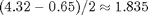$(4.32 - 0.65)/2 \approx 1.835$ . Since the input amplitude is approximately $5/2 = 2.5$ , that means the arrangement'south magnitude at this frequency can exist calculated as follows.

(iii) $\textrm{magnitude} = \frac{Y}{R} \approx \frac{1.835}{2.5} \approx 0.734 \Rightarrow 20\log_{10} \frac{Y}{R} \approx -2.686 \textrm{dB}$

This process can then exist repeated for the 18 other frequencies specified in the table higher up. An example set of raw output response data has been stored here in frequency_response_data.mat. From this data, or your own, y'all can then estimate by hand the magnitude of the system's response at the other 18 frequencies.

The example given above showed that the system adulterate the input somewhat (magnitude less than one) at a frequency of approximately 1.571 rad/sec. This was to be expected since this frequency was slightly greater than the organisation's predicted break frequency. Entering the following code will allow us to examine the organization's response for a slower frequency, specifically, for $T = 40$ seconds which corresponds to a frequency of approximately 0.157 rad/sec.

load          frequency_response_data.mat          figure; plot(0:0.1:100,eo_act_40,0:0.1:100,ei_40,'r') xlabel('time (sec)'); ylabel('signals (Volts)'); title('RC Circuit Foursquare Moving ridge Response for T = 40 sec'); legend('output','input');

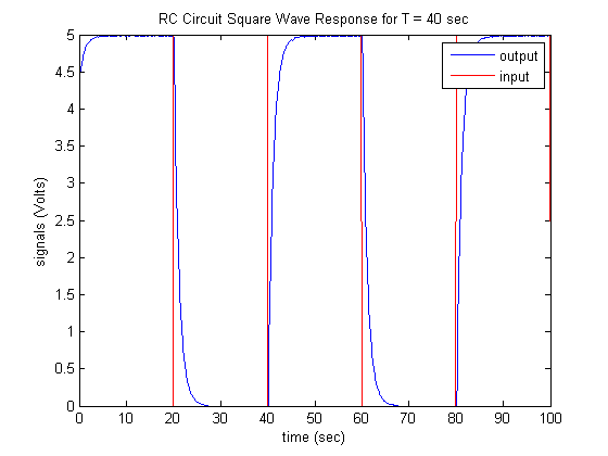
As expected, since the period of the square moving ridge input is then much larger than the RC circuit's time constant, the output response has plenty of time to reach steady state earlier the input switches. Therefore, the circuit's magnitude response at this frequency is approximately 1 (0 dB). When the period equaled 4 seconds, the circuit did not have enough time to reach steady-land, hence the output was somewhat attenuated. If we decrease the menses of the input farther (increase the frequency), the circuit will accept even less time to reply and the output will exist adulterate further. Executing the post-obit commands volition show the circuit's response for an input square wave with period $T = 0.4$ seconds, which corresponds to a frequency of approximately 15.71 rad/sec.

load          frequency_response_data.mat          figure; plot(0:0.02:8,eo_act_dot4(1:401),0:0.02:8,ei_dot4(1:401),'r') xlabel('time (sec)'); ylabel('signals (Volts)'); title('RC Circuit Foursquare Wave Response for T = 0.4 sec'); fable('output','input');

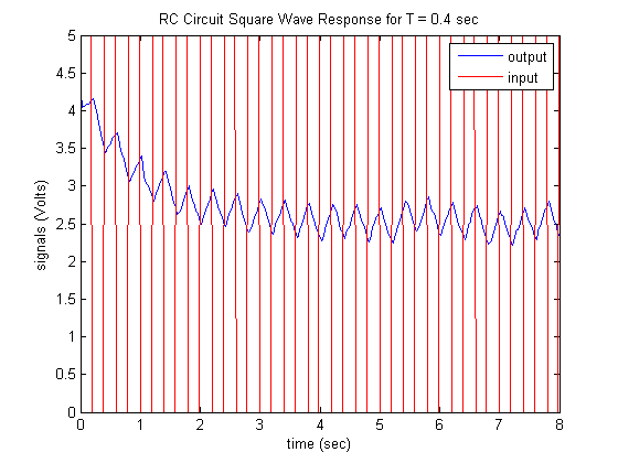
Every bit we expected, the output is much adulterate as compared to the input. Some other affair that you will notice is that the output becomes less stable at these college frequencies. This arises for a couple of reasons. For one, since the output aamplitude is much smaller, any errors or disturbances become a larger percent of the amplitude. 2d, every bit the frequency of the signals increase, a smaller sample time is required to get a sufficient number of points per period in social club to reconstruct the output response. If the signals are sufficiently fast, we will come across the speed limitations of the experimental hardware and software. For the experimental ready-up we are employing, we cannot achieve sample times faster than nearly 0.01 seconds. Therefore, at higher frequencies we may sometimes miss the truthful extremes of the output signal (the peaks and valleys could occur betwixt samples).

In order to construct the Bode magnitude plot we desire, nosotros then need to calculate the gain at each of the 19 frequencies outlined in our original tabular array. This can be performed manually as nosotros demonstrated for $T = 4$ seconds. Alternatively, nosotros tin employ the program plot_mag.one thousand that nosotros accept written to generate the Bode magnitude plot. This plotting script employs the function cal_avg.g to summate the average amplitude of the output response data for each of the prescribed periods. This function presumes the output data is saved with the same name and format as frequency_response_data.mat. Executing the program plot_mag.m will then generate a plot similar the one shown below. Note the magnitude at $\omega = 1.571$ rad/sec ( $T = 4$ seconds) approximately matches the value we calculated by hand ( $\approx -2.686$ dB).

If you calculate the magnitudes manually (in dB) and shop them in the vector M and shop the corresponding frequencies in the vector w, then the following commands volition generate a plot like the one shown above.

          s = tf('south')          R = x*10^three;                                    C = 100*ten^-6;                                  G = i/(R*C*s + 1);                              figure; semilogx(w,One thousand,'r*');          hold          on;          bodemag(G);          legend('experiment','theory','Location','SouthWest')          grid          on;

Inspection of the above Bode plot shows qualitative agreement between the magnitude response predicted by theory and the experimental information we recorded. Some of the divergence can exist attributed to mismatch between the assumed and bodily component values (R and C). Nonetheless, the chief cause of the discrepancy is that nosotros performed our experiments by sweeping through the frequencies of square wave inputs, rather than employing sinusoidal inputs, as is the standard for frequency response analysis. We employed foursquare wave inputs in lodge to build intuition for why a arrangement responds differently to inputs of varying frequencies. Furthermore, nearly models of Arduino board do not have the ability to generate analog outputs.

While nosotros did non construct the phase response portion of the Bode plot for this circuit, the data we recorded does provide some intuition here also. Consider that ane period corresponds to 360 degrees. For a square wave input, nosotros can consider that the wave switches from five Volts to 0 Volts at the 180 degree position in its cycle. Furthermore, we can approximate the wave as reaching its "peak" at the midpoint of its ON land, which would be at the 90 degree position of its cycle. When the foursquare wave input is slow, for instance $T = 40$ seconds, the output reaches 5 Volts relatively apace as compared to the length of the period. As such, the "meridian" of the output wave lags behind the "superlative" of the input wave merely slightly. As the frequency of the input increases, for example $T = 4$ seconds or $T = 0.4$ seconds, the output reaches its maximum value at the point when the input switches from 5 Volts to 0 Volts. Therefore, the output reaches its elevation at the 180 degree position, which is 90 degrees afterwards the input reaches its peak (stage = -90 degrees). This agrees with the theoretical Bode phase plot generated at the offset of this activity.

This behavior also makes intuitive sense. Since it takes time for a physical system to react to a change in its input, the output volition always lag behind the input. The "speed" of the system is in essence constant (the time constant doesn't change), nonetheless, the time it takes a organization to react every bit a percentage of the input's period increases as the input becomes faster. In other words, $\tau$ is the same whether the input has menses $T = 40$ seconds or period $T = 4$ seconds, but $\tau$ becomes a much larger percentage of the period as the frequency increases. This sort of beliefs is indicative of most physical systems in that the output volition lag behind the input to a greater degree every bit the frequency of the input is increased.

Extensions

If you would like to experimentally generate the frequency response of this circuit employing sinusoidal inputs, there are a couple of options. One approach is to use an external function generator to generate the inputs to the RC circuit, rather than generating the input from the Arduino board. Another option is to employ a board that is able to generate analog outputs. Ane such example is the Arduino Due. Most other Arduino models (Uno, Mega 2560, etc.), however, tin can only generate digital outputs. In that example, y'all tin consider the input to the circuit to be the duty cycle of a pulse-width modulated square moving ridge. Therefore, you can observe the frequency response of the excursion by sinusoidally varying the duty cycle beyond dissimilar frequencies. To see an instance of this approach, refer to the system identification experiment performed for a Boost Converter Excursion in Activity 5b.

In Part (c) of this activity, a controller is implemented to change the response characteristics of the RC circuit.

All contents licensed under a Artistic Commons Attribution-ShareAlike 4.0 International License.